Introduction
In this article, directed acyclic graphs (DAGs) from the same equivalence class will be given for the case when the number of features is so big that there will be d-separation implications among the features. That’s the mean, some features will be conditionally independent of some other features given some other features. The reasoning presented in the articles [1] and [2] is followed and expanded in this article.
The Reasoning
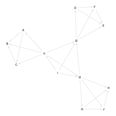
As the number of features in the image increases, new sub-intents will begin to appear. These sub-intents like $I_{1}, I_{2}, I_{3}, …$ will be related with the image’s main intent $I$. Each sub-intent will be connected with some of the features in the image. Features around a sub-intent will be dependent on features around another sub-intent by means of the sub-intents. Therefore, once a sub-intent is conditioned on, the features around this intent will be independent of all other features. A sample DAG is shown in the Figure 1.

In this sample, each sub-intent has three related features. As indicated in [2], the number of maximum features depends on the number of pixels in a feature and the total number of pixels in the image. For the case of the sub-intents, the number of maximum features can be determined using the number of pixels in a related feature and the total number of pixels in the sub-intent region. There are three sub-intents in this sample DAG.
Equivalence Class
The equivalence class of the DAG in the Figure 1 has been found using DAGitty package [3] from R. The DAG drawn by DAGitty is shown in the Figure 2.
The DAGs from the equivalence class of the DAG in the Figure 1 are represented as follows: \begin{equation} \begin{array}{l} \text{pdag} ( \newline A, B, C, D, E, F, G, H, I, I_{1}, I_{2}, I_{3}, J \newline A -- B, A -- C, A -- I_{1}, B -- C, B -- I_{1}, C -- I_{1}, D -- E, D -- F \newline D -- I_{2}, E -- F, E -- I_{2}, F -- I_{2}, G -- H, G -- I_{3}, G -- J, H -- I_{3} \newline H -- J, I -- I_{1}, I -- I_{2}, I -- I_{3}, I_{1} -- I_{2}, I_{1} -- I{3}, I_{2} -- I_{3}, I_{3} -- J \newline ) \end{array} \label{equivalenceClassRep} \end{equation} In the representation given in the equation (\ref{equivalenceClassRep}), the nodes in the equivalent DAGs are listed first. Then, the arrows which can be in any two possible directions are indicated. For example, $A -- B$ means either $A \rightarrow B$ or $A \leftarrow B$. From the equation (\ref{equivalenceClassRep}), it is observed that all of the edges can have either of the possible two directions. Hence, there are a total of $2^{24}$ DAGs in the equivalence class. However, in our image model, edges can only leave the intent nodes which are $I$, $I_{1}$, $I_{2}$ and $I_{3}$. Hence, there are $2^{24}/2^{12}=2^{12}$ DAGs from the same equivalence set for our image model.
d-separation Implications
The d-separation implications in the DAG shown in the Figure 1 has been found using DAGitty. They are listed as follows: \begin{equation} \begin{array}{lllllllll} A \stackrel{||}{\rule{0.3cm}{0.5pt}} D \, | \, I_{2} & A \stackrel{||}{\rule{0.3cm}{0.5pt}} D \, | \, I_{1} & A \stackrel{||}{\rule{0.3cm}{0.5pt}} E \, | \, I_{2} & A \stackrel{||}{\rule{0.3cm}{0.5pt}} E \, | \, I_{1} & A \stackrel{||}{\rule{0.3cm}{0.5pt}} F \, | \, I_{2} & A \stackrel{||}{\rule{0.3cm}{0.5pt}} F \, | \, I_{1} & A \stackrel{||}{\rule{0.3cm}{0.5pt}} G \, | \, I_{3} & A \stackrel{||}{\rule{0.3cm}{0.5pt}} G \, | \, I_{1} & A \stackrel{||}{\rule{0.3cm}{0.5pt}} H \, | \, I_{3} \newline A \stackrel{||}{\rule{0.3cm}{0.5pt}} H \, | \, I_{1} & A \stackrel{||}{\rule{0.3cm}{0.5pt}} I \, | \, I_{1} & A \stackrel{||}{\rule{0.3cm}{0.5pt}} I_{2} \, | \, I_{1} & A \stackrel{||}{\rule{0.3cm}{0.5pt}} I_{3} \, | \, I_{1} & A \stackrel{||}{\rule{0.3cm}{0.5pt}} J \, | \, I_{3} & A \stackrel{||}{\rule{0.3cm}{0.5pt}} J \, | \, I_{1} & B \stackrel{||}{\rule{0.3cm}{0.5pt}} D \, | \, I_{2} & B \stackrel{||}{\rule{0.3cm}{0.5pt}} D \, | \, I_{1} & B \stackrel{||}{\rule{0.3cm}{0.5pt}} E \, | \, I_{2} \newline B \stackrel{||}{\rule{0.3cm}{0.5pt}} E \, | \, I_{1} & B \stackrel{||}{\rule{0.3cm}{0.5pt}} F \, | \, I_{2} & B \stackrel{||}{\rule{0.3cm}{0.5pt}} F \, | \, I_{1} & B \stackrel{||}{\rule{0.3cm}{0.5pt}} G \, | \, I_{3} & B \stackrel{||}{\rule{0.3cm}{0.5pt}} G \, | \, I_{1} & B \stackrel{||}{\rule{0.3cm}{0.5pt}} H \, | \, I_{3} & B \stackrel{||}{\rule{0.3cm}{0.5pt}} H \, | \, I_{1} & B \stackrel{||}{\rule{0.3cm}{0.5pt}} I \, | \, I_{1} & B \stackrel{||}{\rule{0.3cm}{0.5pt}} I_{2} \, | \, I_{1} \newline B \stackrel{||}{\rule{0.3cm}{0.5pt}} I_{3} \, | \, I_{1} & B \stackrel{||}{\rule{0.3cm}{0.5pt}} J \, | \, I_{3} & B \stackrel{||}{\rule{0.3cm}{0.5pt}} J \, | \, I_{1} & C \stackrel{||}{\rule{0.3cm}{0.5pt}} D \, | \, I_{2} & C \stackrel{||}{\rule{0.3cm}{0.5pt}} D \, | \, I_{1} & C \stackrel{||}{\rule{0.3cm}{0.5pt}} E \, | \, I_{2} & C \stackrel{||}{\rule{0.3cm}{0.5pt}} E \, | \, I_{1} & C \stackrel{||}{\rule{0.3cm}{0.5pt}} F \, | \, I_{2} & C \stackrel{||}{\rule{0.3cm}{0.5pt}} F \, | \, I_{1} \newline C \stackrel{||}{\rule{0.3cm}{0.5pt}} G \, | \, I_{3} & C \stackrel{||}{\rule{0.3cm}{0.5pt}} G \, | \, I_{1} & C \stackrel{||}{\rule{0.3cm}{0.5pt}} H \, | \, I_{3} & C \stackrel{||}{\rule{0.3cm}{0.5pt}} H \, | \, I_{1} & C \stackrel{||}{\rule{0.3cm}{0.5pt}} I \, | \, I_{1} & C \stackrel{||}{\rule{0.3cm}{0.5pt}} I_{2} \, | \, I_{1} & C \stackrel{||}{\rule{0.3cm}{0.5pt}} I_{3} \, | \, I_{1} & C \stackrel{||}{\rule{0.3cm}{0.5pt}} J \, | \, I_{3} & C \stackrel{||}{\rule{0.3cm}{0.5pt}} J \, | \, I_{1} \newline D \stackrel{||}{\rule{0.3cm}{0.5pt}} G \, | \, I_{3} & D \stackrel{||}{\rule{0.3cm}{0.5pt}} G \, | \, I_{2} & D \stackrel{||}{\rule{0.3cm}{0.5pt}} H \, | \, I_{3} & D \stackrel{||}{\rule{0.3cm}{0.5pt}} H \, | \, I_{2} & D \stackrel{||}{\rule{0.3cm}{0.5pt}} I \, | \, I_{2} & D \stackrel{||}{\rule{0.3cm}{0.5pt}} I_{1} \, | \, I_{2} & D \stackrel{||}{\rule{0.3cm}{0.5pt}} I_{3} \, | \, I_{2} & D \stackrel{||}{\rule{0.3cm}{0.5pt}} J \, | \, I_{3} & D \stackrel{||}{\rule{0.3cm}{0.5pt}} J \, | \, I_{2} \newline E \stackrel{||}{\rule{0.3cm}{0.5pt}} G \, | \, I_{3} & E \stackrel{||}{\rule{0.3cm}{0.5pt}} G \, | \, I_{2} & E \stackrel{||}{\rule{0.3cm}{0.5pt}} H \, | \, I_{3} & E \stackrel{||}{\rule{0.3cm}{0.5pt}} H \, | \, I_{2} & E \stackrel{||}{\rule{0.3cm}{0.5pt}} I \, | \, I_{2} & E \stackrel{||}{\rule{0.3cm}{0.5pt}} I_{1} \, | \, I_{2} & E \stackrel{||}{\rule{0.3cm}{0.5pt}} I_{3} \, | \, I_{2} & E \stackrel{||}{\rule{0.3cm}{0.5pt}} J \, | \, I_{3} & E \stackrel{||}{\rule{0.3cm}{0.5pt}} J \, | \, I_{2} \newline F \stackrel{||}{\rule{0.3cm}{0.5pt}} G \, | \, I_{3} & F \stackrel{||}{\rule{0.3cm}{0.5pt}} G \, | \, I_{2} & F \stackrel{||}{\rule{0.3cm}{0.5pt}} H \, | \, I_{3} & F \stackrel{||}{\rule{0.3cm}{0.5pt}} H \, | \, I_{2} & F \stackrel{||}{\rule{0.3cm}{0.5pt}} I \, | \, I_{2} & F \stackrel{||}{\rule{0.3cm}{0.5pt}} I_{1} \, | \, I_{2} & F \stackrel{||}{\rule{0.3cm}{0.5pt}} I_{3} \, | \, I_{2} & F \stackrel{||}{\rule{0.3cm}{0.5pt}} J \, | \, I_{3} & F \stackrel{||}{\rule{0.3cm}{0.5pt}} J \, | \, I_{2} \newline G \stackrel{||}{\rule{0.3cm}{0.5pt}} I \, | \, I_{3} & G \stackrel{||}{\rule{0.3cm}{0.5pt}} I_{1} \, | \, I_{3} & G \stackrel{||}{\rule{0.3cm}{0.5pt}} I_{2} \, | \, I_{3} & H \stackrel{||}{\rule{0.3cm}{0.5pt}} I \, | \, I_{3} & H \stackrel{||}{\rule{0.3cm}{0.5pt}} I_{1} \, | \, I_{3} & H \stackrel{||}{\rule{0.3cm}{0.5pt}} I_{2} \, | \, I_{3} & I \stackrel{||}{\rule{0.3cm}{0.5pt}} J \, | \, I_{3} & I_{1} \stackrel{||}{\rule{0.3cm}{0.5pt}} J \, | \, I_{3} & I_{2} \stackrel{||}{\rule{0.3cm}{0.5pt}} J \, | \, I_{3} \end{array} \label{dSepImp1} \end{equation} The d-separation implications in the equation (\ref{dSepImp1}) shows that features around a sub-intent are dependent on the features around another sub-intent by means of the sub-intents. When the sub-intent is conditioned on, the features around the conditioned sub-intent become independent of all the other features in the DAG. For example, the following implications exhibit this independence for the case of the feature $A$: \begin{equation} \begin{array}{lll} A \stackrel{||}{\rule{0.3cm}{0.5pt}} D \, | \, I_{1} & A \stackrel{||}{\rule{0.3cm}{0.5pt}} E \, | \, I_{1} & A \stackrel{||}{\rule{0.3cm}{0.5pt}} F \, | \, I_{1} \newline A \stackrel{||}{\rule{0.3cm}{0.5pt}} G \, | \, I_{1} & A \stackrel{||}{\rule{0.3cm}{0.5pt}} H \, | \, I_{1} & A \stackrel{||}{\rule{0.3cm}{0.5pt}} I \, | \, I_{1} \newline A \stackrel{||}{\rule{0.3cm}{0.5pt}} I_{2} \, | \, I_{1} & A \stackrel{||}{\rule{0.3cm}{0.5pt}} I_{3} \, | \, I_{1} & A \stackrel{||}{\rule{0.3cm}{0.5pt}} J \, | \, I_{1} \end{array} \end{equation}
There is another set of d-separation implications which are in a different form. These are also given as follows: \begin{equation} \begin{array}{l} A \stackrel{||}{\rule{0.3cm}{0.5pt}} D, E, F, G, H, I, I_{2}, I_{3}, J \, | \, I_{1} \newline B \stackrel{||}{\rule{0.3cm}{0.5pt}} D, E, F, G, H, I, I_{2}, I_{3}, J \, | \, A, C, I_{1} \newline C \stackrel{||}{\rule{0.3cm}{0.5pt}} D, E, F, G, H, I, I_{2}, I_{3}, J \, | \, A, I_{1} \newline D \stackrel{||}{\rule{0.3cm}{0.5pt}} A, B, C, G, H, I, I_{1}, I_{3}, J \, | \, I_{2} \newline E \stackrel{||}{\rule{0.3cm}{0.5pt}} A, B, C, G, H, I, I_{1}, I_{3}, J \, | \, D, F, I_{2} \newline F \stackrel{||}{\rule{0.3cm}{0.5pt}} A, B, C, G, H, I, I_{1}, I_{3}, J \, | \, D, I_{2} \newline G \stackrel{||}{\rule{0.3cm}{0.5pt}} A, B, C, D, E, F, I, I_{1}, I_{2} \, | \, I_{3} \newline H \stackrel{||}{\rule{0.3cm}{0.5pt}} A, B, C, D, E, F, I, I_{1}, I_{2} \, | \, G, I_{3}, J \newline I_{2} \stackrel{||}{\rule{0.3cm}{0.5pt}} A, B, C, G, H, J \, | \, I, I_{1}, I_{3} \newline I_{3} \stackrel{||}{\rule{0.3cm}{0.5pt}} A, B, C \, | \, I, I_{1} \newline J \stackrel{||}{\rule{0.3cm}{0.5pt}} A, B, C, D, E, F, I, I_{1}, I_{2} \, | \, G, I_{3} \end{array} \label{dSepImp2} \end{equation} The second set of d-separation implications in the equation (\ref{dSepImp2}) causes the data set to be be divided into many clusters due to the big number of variables in the second variable position in the d-separation implications. The existance of many clusters in the date set decreases the number of samples for testing a d-separation implication. However, there is not such a problem for the case of d-separation implications given in the equation (\ref{dSepImp1}).
Conclusion
DAGs from the same equivalence class have been created for the case when there are d-separation implications among features. DAGs from the equivalence class for a sample DAG has been given. The d-separation implications for this sample DAG have been written down using DAGitty.
References
[2] Johannes Textor, Benito van der Zander, Mark K. Gilthorpe, Maciej Liskiewicz, George T.H. Ellison. Robust causal inference using directed acyclic graphs: the R package ‘dagitty’. International Journal of Epidemiology 45(6):1887-1894, 2016.