Introduction
There is an $M \times N$ black and white image. The black pixels are represented by $-1$ whereas the white pixels are denoted by $1$. The image is divided into $m\times n$ blocks. The aim is to find a filter of the same size as the blocks, i.e. $m\times n$. The inner product of the filter with a block should yield a number which is unique to the block. So, a one-to-one mapping between an image and the filter is to be found.
The Solution
I cannot solve this problem analytically. Therefore, I solve it numerically using gradient descent optimization. First, I create all the permutations of $\left\lbrace-1, 1\right\rbrace$ on the $m\times n$ block. The related Python code for a $3\times 2$ filter is as follows:
# possible values of the pixels
g = [-1, 1]

# number of pixels of the filter
gridSize = 6
# all the permutations of -1 and 1 on the block of size gridSize. the number
# of permutations is 2 to the power of gridSize.
permutations = np.array(list(product(g, repeat=gridSize)))
The permutations can be found using the function “product” from “itertools” package. The number of permutations is 2 to the power of number of pixels of the filter.
For creating a filter the inner products of which with the blocks yield unique numbers, the difference of any permutation from any other permutation must be nonzero. Let an example be given. Two permutations $p_{1}$ and $p_{2}$ of 64 possible ones are written as matrices as follows: \begin{equation} p_{1}= \begin{bmatrix} c_{11} & c_{12} \newline c_{21} & c_{22} \newline c_{31} & c_{32} \end{bmatrix}, \ p_{2}= \begin{bmatrix} d_{11} & d_{12} \newline d_{21} & d_{22} \newline d_{31} & d_{32} \end{bmatrix} \end{equation} Let the $3 \times 2$ filter be written as follows: \begin{equation} f= \begin{bmatrix} f_{11} & f_{12} \newline f_{21} & f_{22} \newline f_{31} & f_{32} \end{bmatrix} \end{equation} The inner product of $f$ and $p_{1}$, $<f, p_{1}>$, and the inner product of $f$ and $p_{2}$, $<f, p_{2}>$, are calculated as follows: \begin{gather} <f, p_{1}>=c_{11}f_{11}+c_{12}f_{12}+c_{21}f_{21}+c_{22}f_{22}+c_{31}f_{31}+ c_{32}f_{32} \newline <f, p_{2}>=d_{11}f_{11}+d_{12}f_{12}+d_{21}f_{21}+d_{22}f_{22}+d_{31}f_{31}+ d_{32}f_{32} \end{gather} The difference between these inner products is given as \begin{equation} <f, p_{1}>-<f, p_{2}> = \left(c_{11}-d_{11}\right)f_{11} + \left(c_{12}-d_{12}\right)f_{12} + \left(c_{21}-d_{21}\right)f_{21} + \left(c_{22}-d_{22}\right)f_{22} + \left(c_{31}-d_{31}\right)f_{31} + \left(c_{32}-d_{32}\right)f_{32} \label{sampleDiff} \end{equation} If this difference is nonzero, then it means that the filter $f$ generates unique identity numbers for $p_{1}$ and $p_{2}$ respectively. All possible values of the difference coefficients of $f_{11}$, $f_{12}$, $f_{21}$, $f_{22}$, $f_{31}$ and $f_{32}$ in the equation \eqref{sampleDiff} are found by means of the following Python code.
# the difference between a permutation and the other permutations are
# computed. each set of differences form a matrix and each matrix is put into a
# list.
theSize = 0
diffList = []
for i in range(permutations.shape[0]-1):
    theVec = permutations[i, :]
    theDiff = theVec-permutations[i+1:, :]
    theSize = theSize + theDiff.shape[0]
    diffList.append(theDiff)
All the values of difference coefficients are then collected in a matrix.
# the matrices in the list are concatenated and collected in a matrix.
theDiffMatrix = np.ones((theSize, gridSize))
startRow = 0
for i in range(len(diffList)):
    currentMatrix = diffList[i]
    stopRow = startRow + currentMatrix.shape[0]
    theDiffMatrix[startRow:stopRow, :] = currentMatrix
    startRow = startRow + currentMatrix.shape[0]
The matrix containing all possible values of the difference coefficients may have duplicate rows. These duplicate rows are removed.
# the difference matrix can have duplicate rows. they are removed.
reducedDiffMatrix, indices = np.unique(theDiffMatrix, axis=0, return_index=True
How will the filter which will generate unique identity numbers for the binary image be found? There is the reducedDiffMatrix which have all possible values of the difference coefficients. First, the filter vector is randomly set. The randomly-set filter is to be tuned to a suitable filter using gradient descent optimization algorithm. The inner product of the filter with every row of the reducedDiffMatrix is done. The inner products which are smaller than or equal to the set threshold which is $0.2$ are determined. The difference coefficients corresponding to these inner products will determine the gradient direction. The related Python code is as follows:
# First, a random filter is created. The filter is updated until one-to-one
# correspondence is satisfied. let a random filter be generated
rng = np.random.default_rng(seed=4)
randFloatVec = rng.random(gridSize)
print("initial random filter:")
print(randFloatVec)
# the inner product of the filter with each row of the reduced difference
# matrix is performed.
innerProducts = np.sum(reducedDiffMatrix * randFloatVec, axis=1)
# the inner products whose values are within a particular neighborhood
# of 0 are determined. Let the radius of the neightborhood be set.
neighRadius = 0.2
# the inner products in the neighborhood are found.
directionIndices  = np.argwhere(np.abs(innerProducts) <= neighRadius).flatten()
Let there be $s$ differences whose values are less than or equal to the set threshold. The filter coefficients should be updated in such a way that these differences increase to exceed the set threshold. The gradient descent logic can determine how the filter coefficients should be updated. Let the $i^{th}$ difference be denoted as $d_{i}$ and written as follows: \begin{equation} d^{i}= d^{i}_{11}f_{11}+d^{i}_{12}f_{12}+d^{i}_{21}f_{21}+d^{i}_{22}f_{22} + d^{i}_{31}f_{31}+d^{i}_{32}f_{32} \end{equation} The gradient of $d^{i}$ with respect to the filter is calculated as in the following: \begin{gather} \nabla_{f} d^{i}= \hat{a}_{f_{11}} \frac{\partial d^{i} }{\partial f_{11}} + \hat{a}_{f_{12}}\frac{\partial d^{i}}{\partial f_{12}} + \hat{a}_{f_{21}}\frac{\partial d^{i} }{\partial f_{21}} + \hat{a}_{f_{22}}\frac{\partial d^{i} }{\partial f_{22}} + \hat{a}_{f_{31}}\frac{\partial d^{i} }{\partial f_{31}} + \hat{a}_{f_{32}}\frac{\partial d^{i} }{\partial f_{32}} \implies \newline \nabla_{f} d^{i} = \hat{a}_{f_{11}} d^{i}_{11}+ \hat{a}_{f_{12}} d^{i}_{12}+ \hat{a}_{f_{21}} d^{i}_{21}+ \hat{a}_{f_{22}} d^{i}_{22}+ \hat{a}_{f_{31}} d^{i}_{31}+ \hat{a}_{f_{32}} d^{i}_{32} \end{gather} In order to increase this $i^{th}$ difference, the filter coefficients must be updated in the direction of this gradient. The information for the resultant update direction comes from the sum of these $s$ gradients assuming that there are $s$ differences whose values are less than or equal to the set threshold. The filter coefficients are updated in the direction of the resultant sum. The related code is as follows:
# the corresponding rows of the reduced difference matrix are gotten.
unnormalizedGradDirections= reducedDiffMatrix[directionIndices]
norms = np.linalg.norm(unnormalizedGradDirections)
gradDirections = unnormalizedGradDirections / norms
# the unnormalized direction is the sum of these rows.
unnormalizedDirection = np.sum(gradDirections, axis=0)
# the normalized direction is calculated.
theDirection = unnormalizedDirection / np.linalg.norm(unnormalizedDirection)
# the update of the filter is done according to the gradient descent logic.
randFloatVec = randFloatVec + stepSize * theDirection
Updating the filter coefficients goes on until there are no differences whose values are less than or equal to the set threshold.
The algorithm explained so far was implemented. The results obtained are to be presented. The filter coefficients are first randomly assigned. The seed for the random assignments is set for reproducibility of results. For the presented results, the following value assignments were made:
- The minimum distance among the unique identities given by the filter to the image blocks is $0.2$.
- The seed is set to $4$.
- The update step size is set to $0.01$.
- The number of coefficients in the filter is $6$.
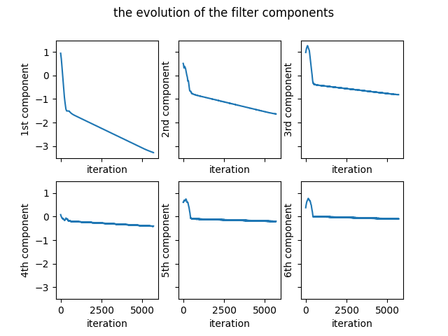
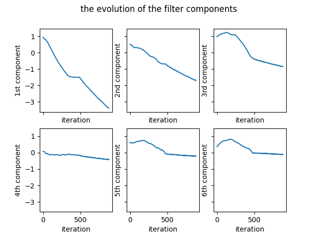
The evolution of the coefficients of the filter is given in the Figure 1.
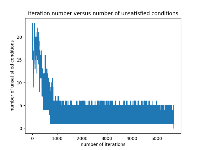
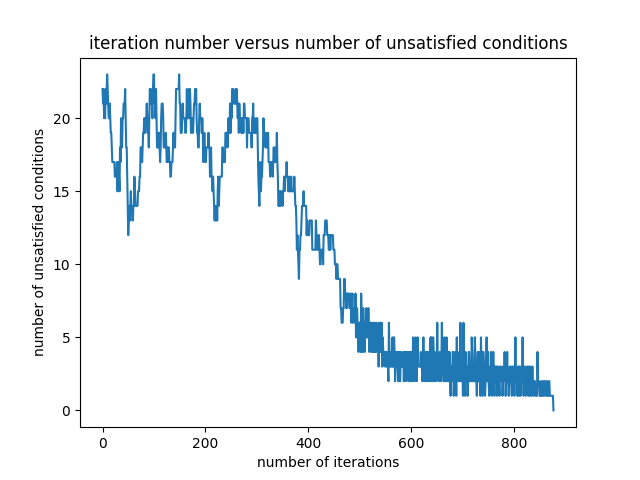
The number of differences which are smaller than the set threshold varies as the optimization goes on. When the number of such differences becomes zero, the optimization ends. The variation of the number of problematic differences is presented in the Figure 2. As can be seen from the figure, as soon as the number of problematic differences becomes zero, the optimization finishes.
The initial random filter for the seed value of $4$ is as follows: \begin{equation} \begin{bmatrix} 0.94305611 & 0.51132755 & 0.97624371 & 0.08083602 & 0.60735583 & 0.37648658 \end{bmatrix} \label{initialFilter} \end{equation} The final filter is as follows: \begin{equation} \begin{bmatrix} -3.2770412 & -1.63632636 & -0.81635904 & -0.40486238 & -0.20267315 & -0.10117016 \end{bmatrix} \label{finalFilter1} \end{equation} The optimization ends after 5680 iterations. There are $64$ permutations of $3\times 2$ image blocks. The unique identity numbers given by the filter to the permutations are as follows: \begin{equation} \begin{matrix} 6.43843228 & 6.23609197 & 6.03308597 & 5.83074566 & 5.62870752 & 5.42636721 & 5.22336122 & 5.0210209 \newline 4.8057142 & 4.60337389 & 4.4003679 & 4.19802759 & 3.99598945 & 3.79364913 & 3.59064314 & 3.38830283 \newline 3.16577956 & 2.96343925 & 2.76043326 & 2.55809295 & 2.3560548 & 2.15371449 & 1.9507085 & 1.74836819 \newline 1.53306149 & 1.33072118 & 1.12771518 & 0.92537487 & 0.72333673 & 0.52099642 & 0.31799043 & 0.11565012 \newline -0.11565012 & -0.31799043 & -0.52099642 & -0.72333673 & -0.92537487 & -1.12771518 & -1.33072118 & -1.53306149 \newline -1.74836819 & -1.9507085 & -2.15371449 & -2.3560548 & -2.55809295 & -2.76043326 & -2.96343925 & -3.16577956 \newline -3.38830283 & -3.59064314 & -3.79364913 & -3.99598945 & -4.19802759 & -4.4003679 & -4.60337389 & -4.8057142 \newline -5.0210209 & -5.22336122 & -5.42636721 & -5.62870752 & -5.83074566 & -6.03308597 & -6.23609197 & -6.43843228 \end{matrix} \label{ids1} \end{equation} It can be observed that the differences between identity numbers are greater than $0.2$. The complete Python code can be found in here.
The differences have varying magnitudes. It will be logical to give more importance to differences of lower magnitudes in the determination of the total gradient. So, as an improvement to the optimization algorithm, a weighing mechanism is incorporated. The less the magnitude of the difference is, the more the related direction is given weight. Therefore, the importance given to the direction corresponding to a difference is inversely proportional to the difference magnitude. The application of weights is performed by the following code snippet:
# find the norms of the inner products which do not satisfy one-to-one
# mapping conditions.
smallMags = allMags[directionIndices]
# weights to be applied to the problematic directions are calculated.
smallMags = np.reshape(allMags[directionIndices], (-1, 1))
# the corresponding rows of the reduced difference matrix are gotten.
unnormalizedGradDirections = reducedDiffMatrix[directionIndices]
norms = np.linalg.norm(unnormalizedGradDirections)
gradDirections = unnormalizedGradDirections / norms
# the weights are applied to the problematic directions.
gradDirections = gradDirections / smallMags
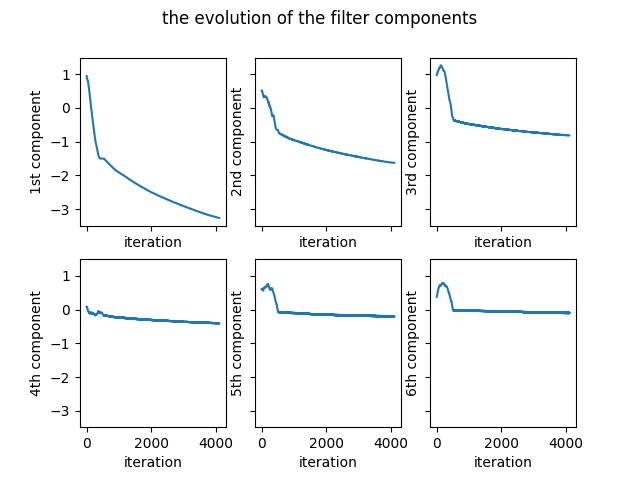
The complete Python code can be found here. The evolution of the coefficients of the filter is given in the Figure 3.
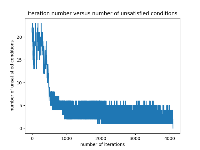
The variation of the number of problematic differences is presented in the Figure 4.
Starting with the same initial random filter as the one given in the equation \eqref{initialFilter}, the final filter is obtained as follows: \begin{equation} \begin{bmatrix} -3.26105616 & -1.62857879 & -0.81504524 & -0.4069397 & -0.20508852 & -0.10086829 \end{bmatrix} \label{finalFilter2} \end{equation} The final filter in the equation \eqref{finalFilter2} is close to the one in the equation \eqref{finalFilter1}.
The optimization ends after 4097 iterations. The unique identity numbers given by the filter to the permutations are as follows: \begin{equation} \begin{matrix} 6.41757669 & 6.21584011 & 6.00739966 & 5.80566308 & 5.6036973 & 5.40196072 \newline 5.19352026 & 4.99178368 & 4.78748622 & 4.58574964 & 4.37730918 & 4.1755726 \newline 3.97360683 & 3.77187025 & 3.56342979 & 3.36169321 & 3.16041911 & 2.95868253 \newline 2.75024207 & 2.54850549 & 2.34653972 & 2.14480313 & 1.93636268 & 1.7346261 \newline 1.53032864 & 1.32859206 & 1.1201516 & 0.91841502 & 0.71644924 & 0.51471266 \newline 0.30627221 & 0.10453563 & -0.10453563 & -0.30627221 & -0.51471266 & -0.71644924 \newline -0.91841502 & -1.1201516 & -1.32859206 & -1.53032864 & -1.7346261 & -1.93636268 \newline -2.14480313 & -2.34653972 & -2.54850549 & -2.75024207 & -2.95868253 & -3.16041911 \newline -3.36169321 & -3.56342979 & -3.77187025 & -3.97360683 & -4.1755726 & -4.37730918 \newline -4.58574964 & -4.78748622 & -4.99178368 & -5.19352026 & -5.40196072 & -5.6036973 \newline -5.80566308 & -6.00739966 & -6.21584011 & -6.41757669 \end{matrix} \label{ids2} \end{equation} The unique identities in the equation \eqref{ids2} are similar to the ones in the equation \eqref{ids1}. It can be observed that the differences between identity numbers are greater than $0.2$.
Another improvement to the optimization algorithm is adding momentum. The momentum is added as shown in the following code snippet:
# the momentum is included
theDirection = theDirection + mu * b
where “b” contains the accumulation of the previous gradients and “mu” is the momentum constant. The complete Python code can be found in here. The evolution of the coefficients of the filter is given in the Figure 5.
The variation of the number of problematic differences is presented in the Figure 6.
Starting with the same initial random filter as the one given in the equation \eqref{initialFilter}, the final filter is obtained as follows: \begin{equation} \begin{bmatrix} -3.37984328 & -1.69863671 & -0.83552461 & -0.40841674 & -0.20248713 & -0.10095605 \end{bmatrix} \label{finalFilter3} \end{equation} The final filter in the equation \eqref{finalFilter3} is close to the one in the equation \eqref{finalFilter1}.
The optimization ends after 877 iterations. The unique identity numbers given
by the filter to the permutations are as follows:
\begin{equation}
\begin{matrix}
6.62586452& 6.42395241& 6.22089027& 6.01897816& 5.80903105& 5.60711894 \newline
5.40405679& 5.20214468& 4.9548153& 4.75290319& 4.54984104& 4.34792893 \newline
4.13798183& 3.93606972& 3.73300757& 3.53109546& 3.22859111& 3.026679 \newline
2.82361685& 2.62170474& 2.41175763& 2.20984552& 2.00678337& 1.80487127 \newline
1.55754188& 1.35562977& 1.15256763& 0.95065552& 0.74070841& 0.5387963 \newline
0.33573415& 0.13382204& -0.13382204& -0.33573415& -0.5387963& -0.74070841 \newline
-0.95065552&-1.15256763&-1.35562977&-1.55754188&-1.80487127&-2.00678337 \newline
-2.20984552&-2.41175763&-2.62170474&-2.82361685& -3.026679& -3.22859111 \newline
-3.53109546&-3.73300757&-3.93606972&-4.13798183&-4.34792893&-4.54984104 \newline
-4.75290319&-4.9548153& -5.20214468&-5.40405679&-5.60711894& -5.80903105 \newline
-6.01897816 & -6.22089027 & -6.42395241 & -6.62586452
\end{matrix}
\end{equation}
It can be observed that the differences between identity numbers are
greater than the set threshold $0.2$.
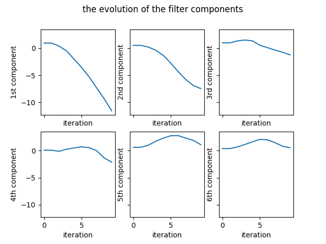
The last improvement to the algorithm is using the Nesterov momentum. How the Nesterov momentum is included in the optimization can be found in here. The evolution of the coefficients of the filter is shown in the Figure 7.
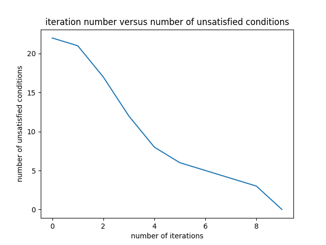
The variation of the number of problematic differences is presented in the Figure 8.
Starting with the same initial random filter as the one given in the equation \eqref{initialFilter}, the final filter is obtained as follows: \begin{equation} \begin{bmatrix} -11.56173079 & -7.47302609 & -1.23863787 & -2.12822715 & 1.09142224 & 0.52917065 \end{bmatrix} \label{finalFilter4} \end{equation} The final filter in the equation \eqref{finalFilter4} is very different from the previous three filters.
The optimization ends after 9 iterations. The unique identity numbers given by
the filter to the permutations are as follows:
\begin{equation}
\begin{matrix}
20.78102901 & 21.8393703 & 22.96387349 & 24.02221479 & 16.52457471 & 17.582916 \newline
18.70741919 & 19.76576048 & 18.30375328 & 19.36209457 & 20.48659776 & 21.54493905 \newline
14.04729898 & 15.10564027 & 16.23014346 & 17.28848475 & 5.83497682 & 6.89331812 \newline
8.0178213 & 9.0761626 & 1.57852252 & 2.63686381 & 3.761367 & 4.8197083 \newline
3.35770109 & 4.41604238 & 5.54054557 & 6.59888686 & -0.89875321 & 0.15958808 \newline
1.28409127 & 2.34243256 & -2.34243256 & -1.28409127 & -0.15958808 & 0.89875321 \newline
-6.59888686 & -5.54054557 & -4.41604238 & -3.35770109 & -4.8197083 & -3.761367 \newline
-2.63686381 & -1.57852252 & -9.0761626 & -8.0178213 & -6.89331812 & -5.83497682 \newline
-17.28848475 & -16.23014346 & -15.10564027 & -14.04729898 & -21.54493905 & -20.48659776 \newline
-19.36209457 & -18.30375328 & -19.76576048 & -18.70741919 & -17.582916 & -16.52457471 \newline
-24.02221479 & -22.96387349 & -21.8393703 & -20.78102901
\end{matrix}
\end{equation}
It can be easily verified that the differences between identity numbers are
greater than the set threshold 0.2.
Conclusion
Several optimization algorithms have been developed and implemented to find a one-to-one mapping between a binary image and a filter of the same size. The inner product of the image and the filter yields a number unique to the image. Due to this uniqueness, the one-to-one mapping is established. Some results from the implementations of the optimization algorithms have been presented.